Image Warping and Mosaicing

Recovering Homographies

The first goal of this project was to write function computeH(im1_pts, im2_pts), which will get us the homography matrix H that tranforms the points in img1 to the points in img2. I used the approach described below.

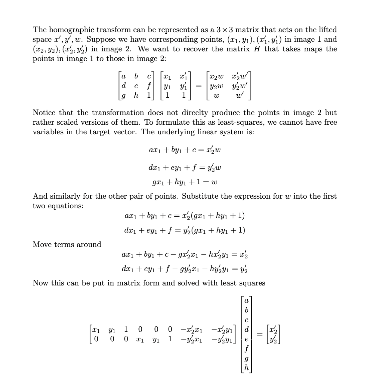
Because there are 8 unknowns, we need at least 4 points on each picture to solve for H. However, having only 4 points can make our data unstable. I used 6-8 points per picture when mosaicing, vertically stacking each new point on the A matrix of the last equation above (2 rows per point). Because we have more values than unknowns, I then dervied a least squares solution to hopefully get an H less prone to noise.

Image Rectification

After computing H, we have all the information we need to warp images. I first tranformed all 4 corners of the image via H to understand the dimensions of the resulting bounding box. Once I had these dimensions, I could create a polygon encapsulting all of the pixels in the resulting image. From here, I used inverse warping to fill in the new image.

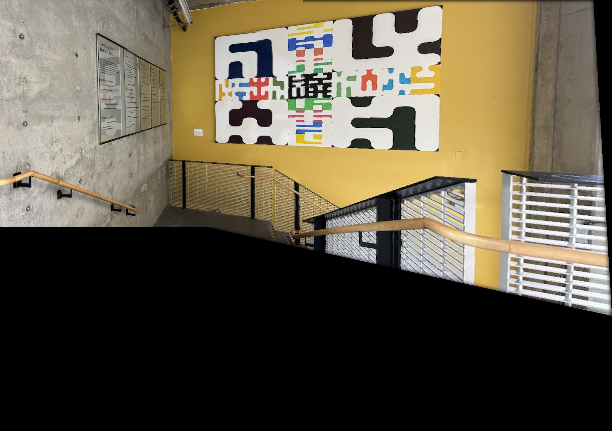
One type of image warping done was image rectification. Here, I corresponded the 4 corners of the rectangular objects in the picture with self-defined rectangular points. This resulted in "straightened out" images.

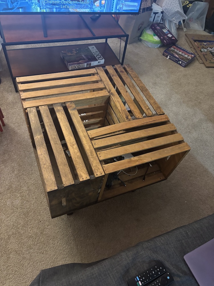
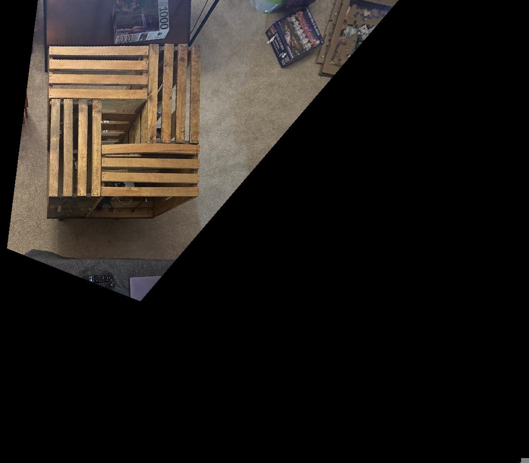
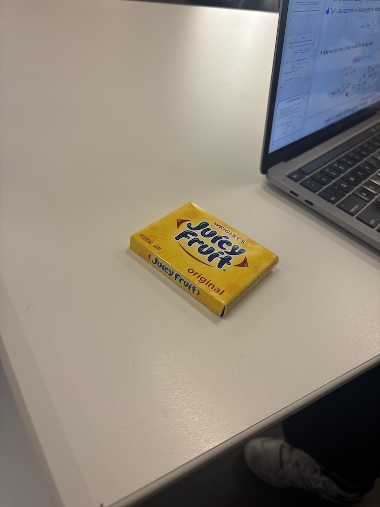
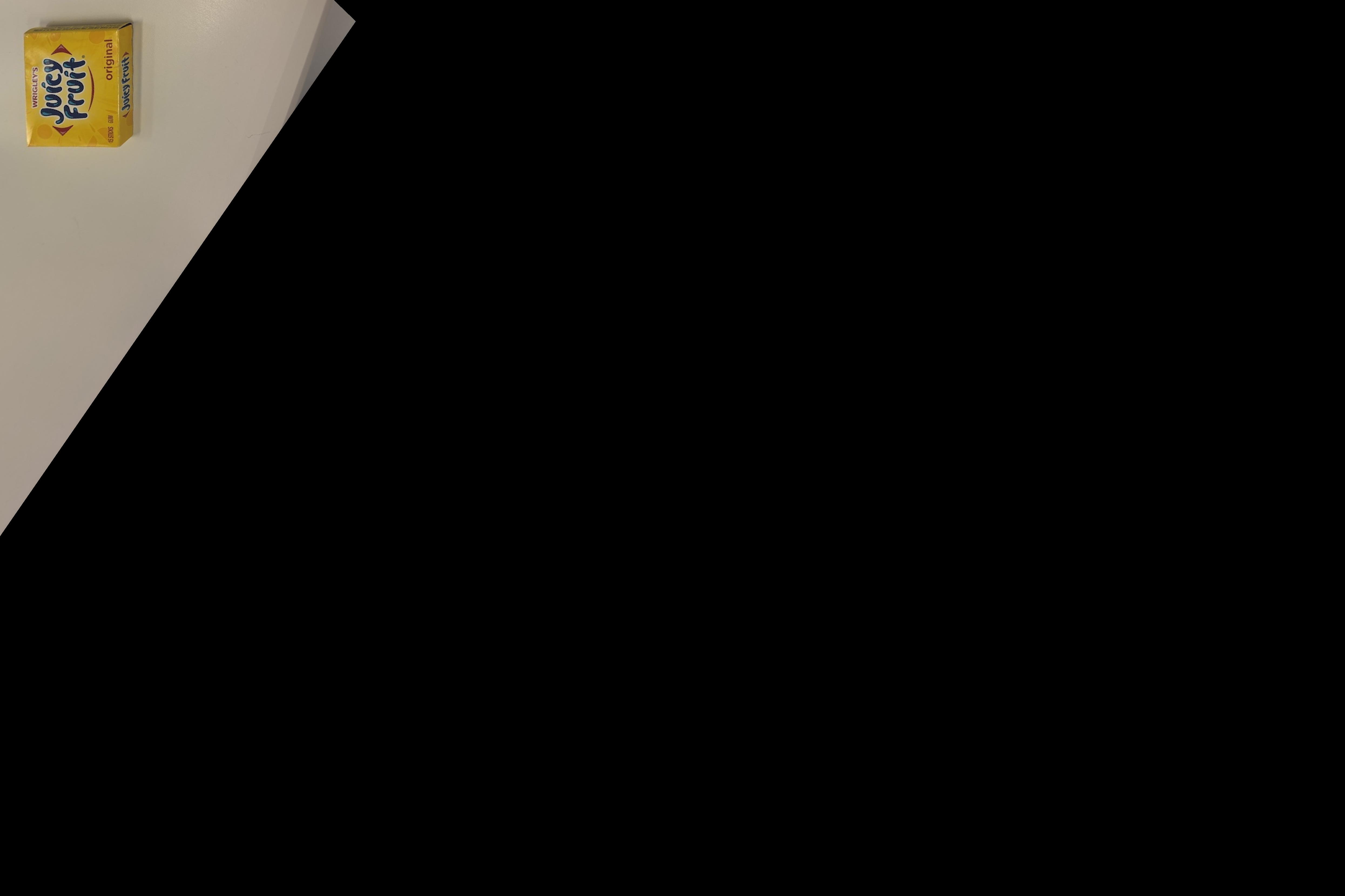
These images had weird cropping because I was manually choosing the tranformation points, and it was difficult to estimate where the rectanlge should end up in the image.

Blending Images into Mosaic

For multiple pics with the same center of projection, I could then blend them into a mosaic.

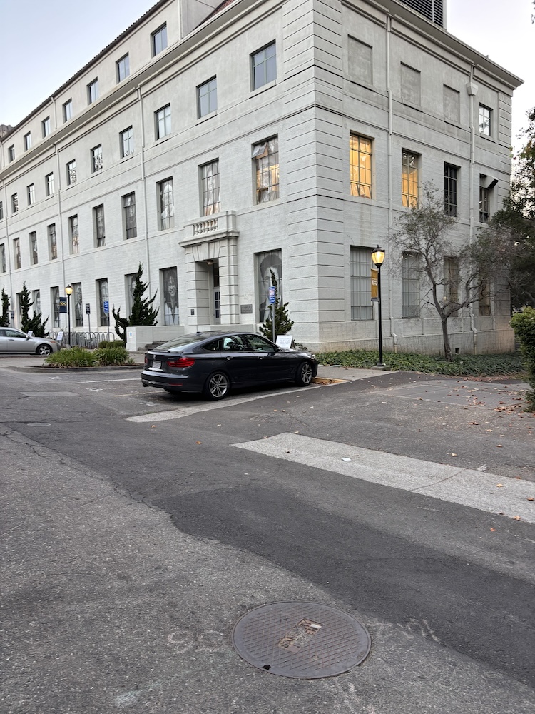
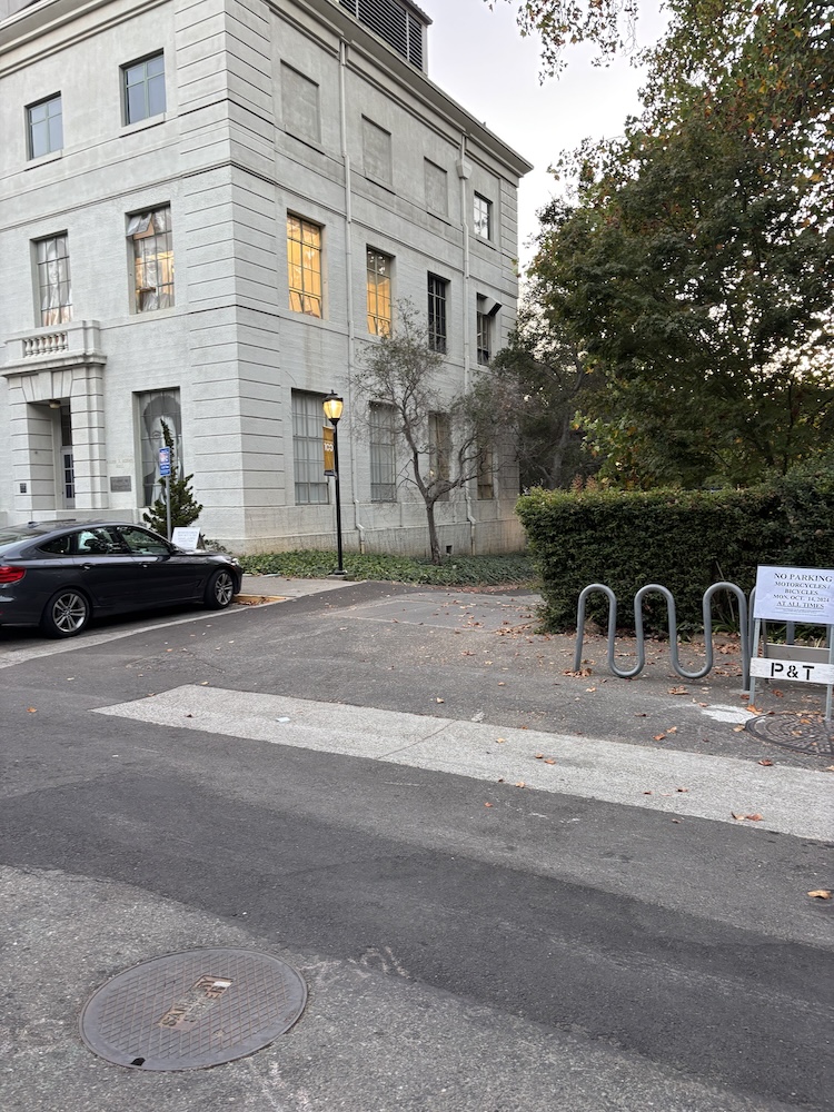
First, I warped one image onto another, and then individually put both the warped and unwarped images onto a matrix of the final mosaic size.

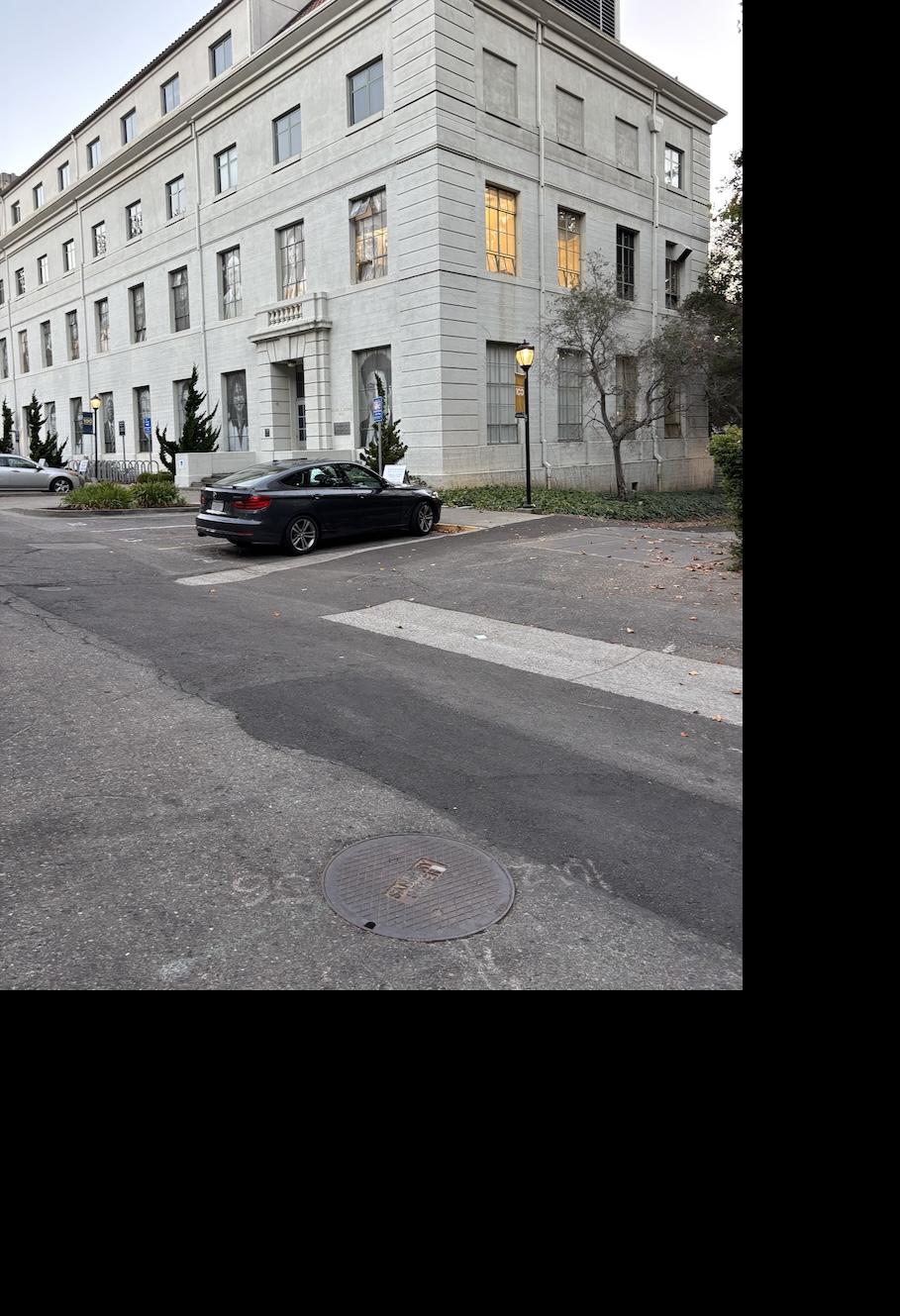
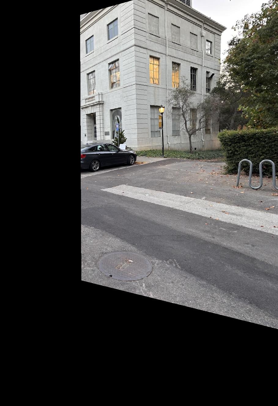
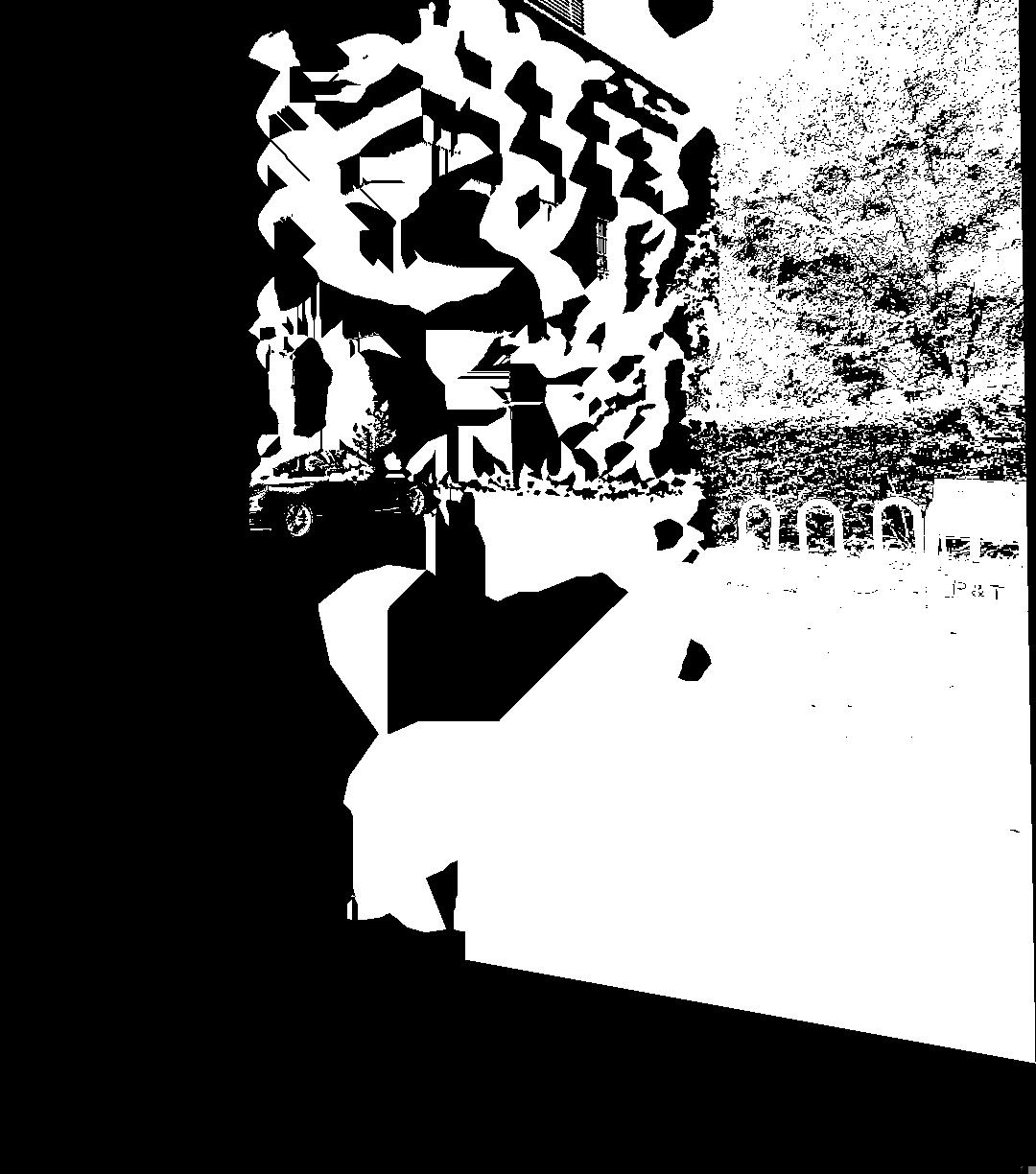
For blending, I used cv2.distanceTransform to create "distance maps" of each pixel in the image to the nearest zero pixel. I then used these two maps to create a mask by only using the values where the distance was greater for the warped image.

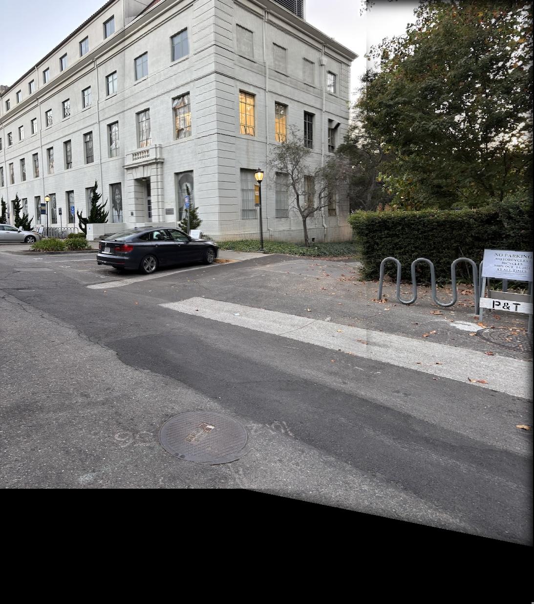
From there, I used Laplacian blending like in Project 2, adding the two images together to create a mosaic.

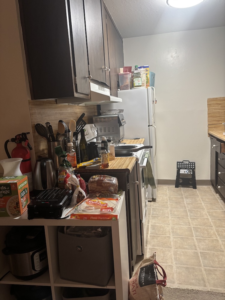
More Examples

Automatic Alignment

To start the process of automatically stitching images together, we needed to identify the Harris corners of each of our images. I used a threshold of 0.05, which I found gave me enough points to work with without being too computationally expensive down the line.

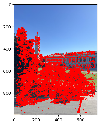
You can see that the sky doesn't have any Harris points here. This is because the sky is a smooth gradient in this pictures with no differentiating features (i.e clouds). It would be extremely difficult to stitch our images based on points in the sky. That being said, if I had lowered my threshold, I would have gotten some points in the sky as well.

Adaptive Non-Maximal Suppression

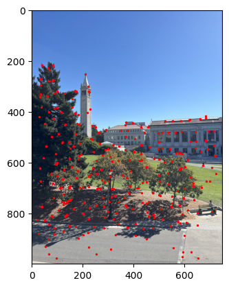
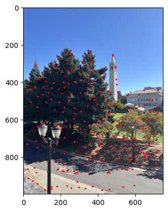
I then implemented ANMS, which filtered down the Harris corners into stronger points that were also spread out. For each of my Harris corners, I found the minimum radius where a robustified point (0.9 * point) with a higher corner strength also exists. Below is the result of the 200 point with the highest radii.

Extracting Feature Descriptors

For each of my ANMS points, I downscaled a 40x40 patch into an 8x8 patch, and normalized it to a mean of 0 and a standard deviation as 1. These will serve as the feature descriptors to then match up points across images.

Matching Feature Descriptors

To match feature descriptors, I implemented a nearest neighbors algorithm that found 1_NN and 2_NN for each ANMS point, which is the closest and second-closest cooresponding point on the other image respectively. To choose the strongest of these points, I set a threshold of 0.25 and only kept a pair of corresponding points if 1_NN/2_NN was less than this threshold.

This is because if the points are indeed a match, 1_NN is likely to have a very low error and 2_NN will have much higher error, so the threshold allows this point to pass. If the points are not a match, the magnitudes of "wrongness" are likely to be more similar.

RANSAC

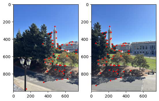
Finally, I used 4-point RANSAC with 1000 iterations to filter out outliers. I used a threshold value of 5. The RANSAC algorithm then uses least-squares on the largest inlier set to get the homography matrix, and we can once again blend the images.

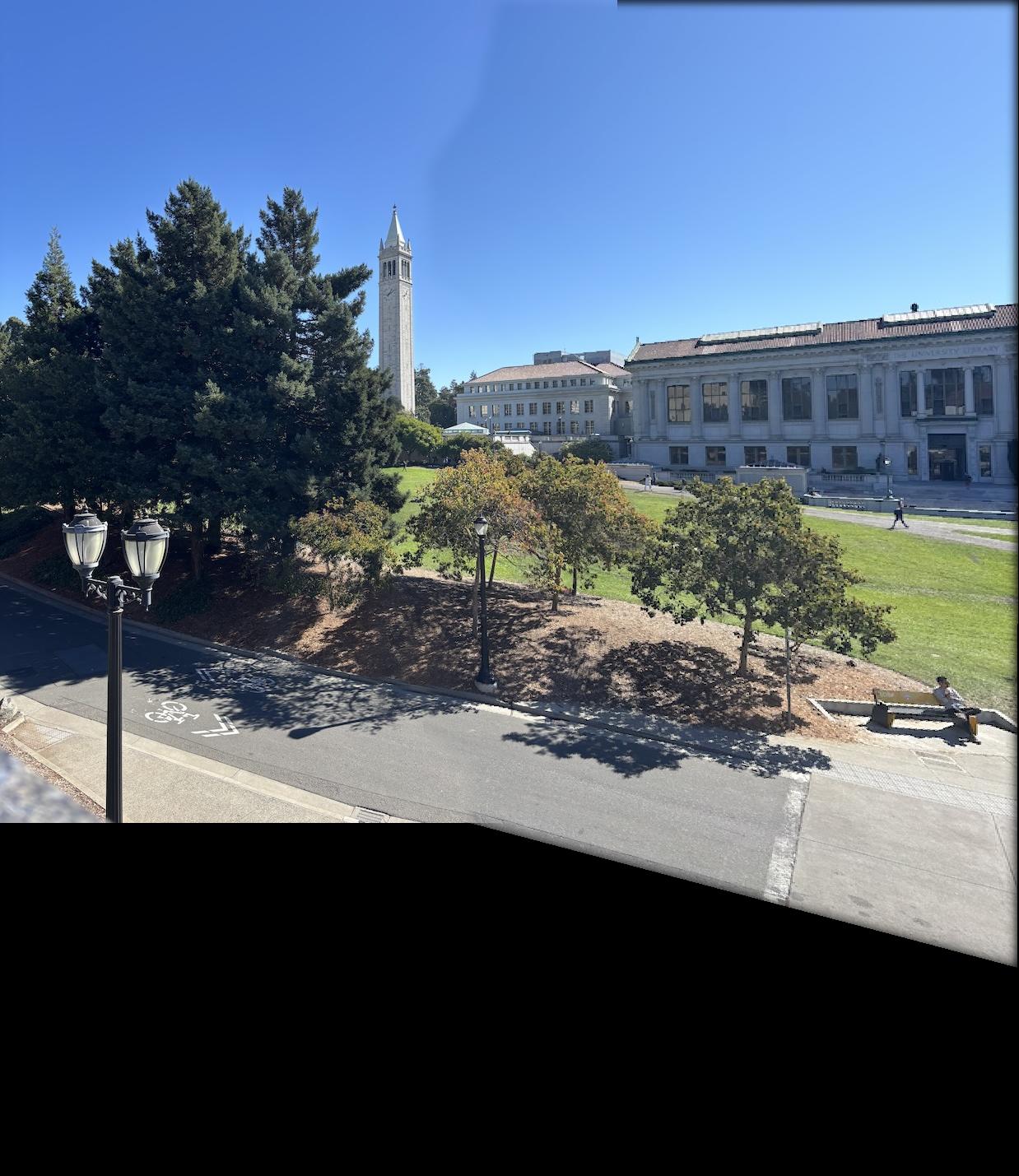
There is a bit of a weird line in the middle of the sky, but I think this is due to the lighting being slightly different in both pictures.

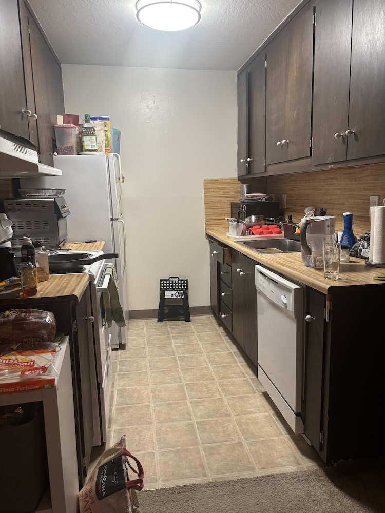
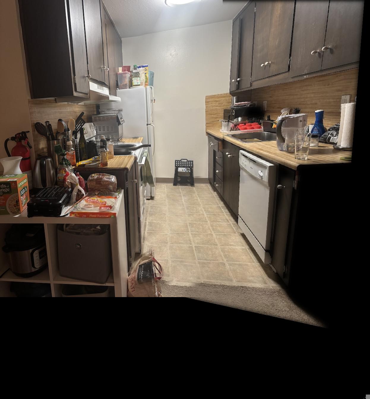
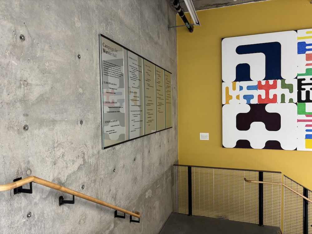
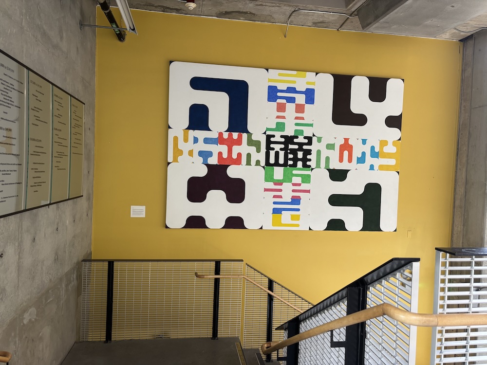
More Examples

The automatic stitching did better than my manual stitching!

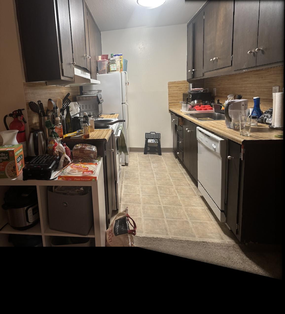
You can see better results in the automatic stithcing, especially where the tile meets the carpet.

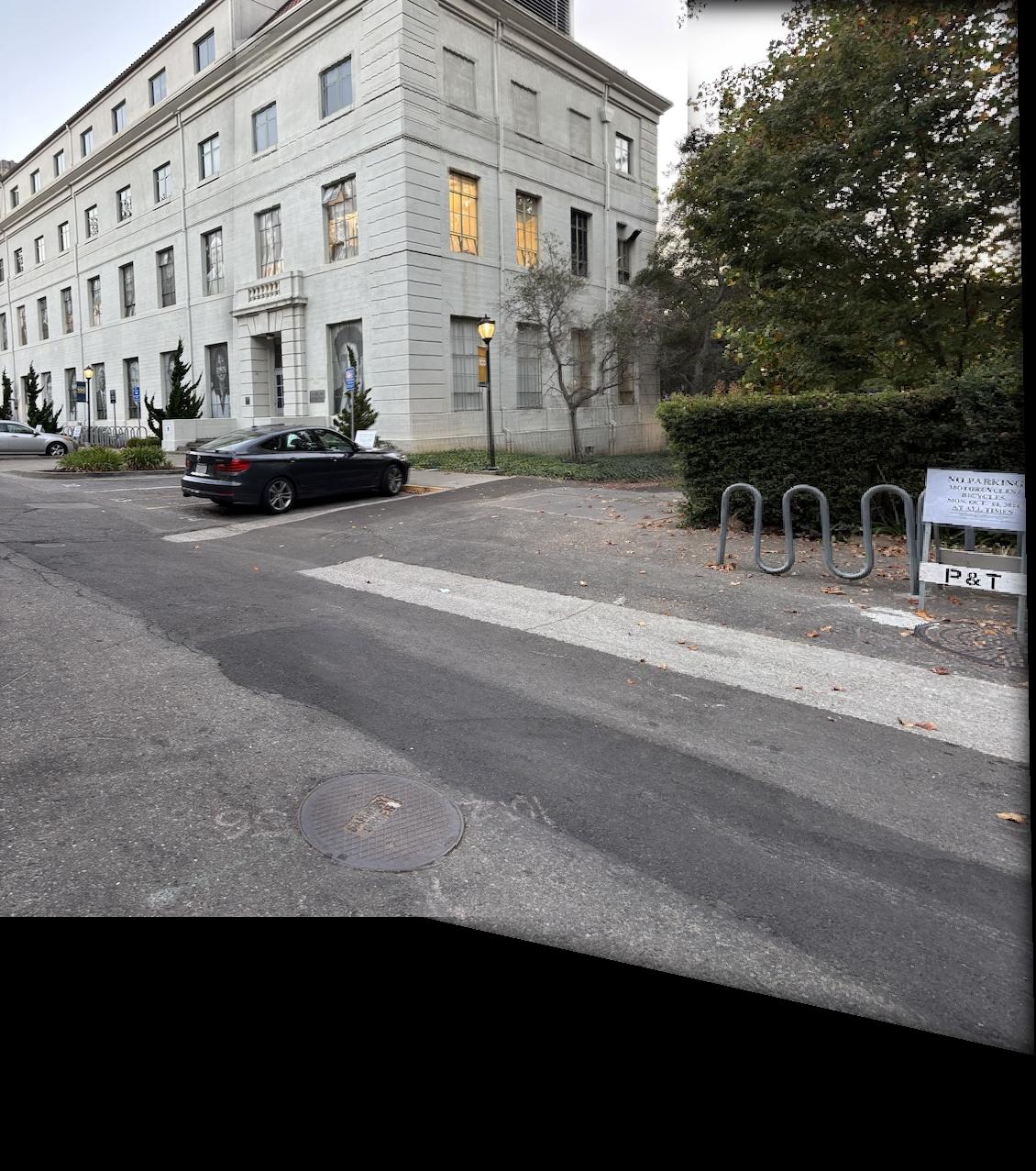
The corner of the building looks less "wavy" in the automatically stitched images. The image on the right is also less blurry in the middle.

Reflection

The coolest thing I learned during this project was the process of matching feature descriptors. I thought the math behind the thresholding was interesting and it's mindblowing that most of the points will line up using this method!